Arc tangente

En mathématiques, l’arc tangente d'un nombre réel est la valeur d'un angle orienté dont la tangente vaut ce nombre.

La fonction qui à tout nombre réel associe la valeur de son arc tangente en radians est la réciproque de la restriction de la fonction trigonométrique tangente à l'intervalle ${\displaystyle \left]-{\frac {\pi }{2}},{\frac {\pi }{2}}\right[}$. La notation est arctan ou Arctan (on trouve aussi Atan, arctg en notation française ; atan ou tan⁻¹, en notation anglo-saxonne (Attention de bien écrire : ${\displaystyle {\frac {1}{\tan x}}=(\tan x)^{-1}}$ et non ${\displaystyle \tan ^{-1}(x)}$).

Pour tout réel x :

${\displaystyle y=\arctan x\iff \tan y=x{\text{ et }}y\in \left]-{\frac {\pi }{2}},{\frac {\pi }{2}}\right[}$.

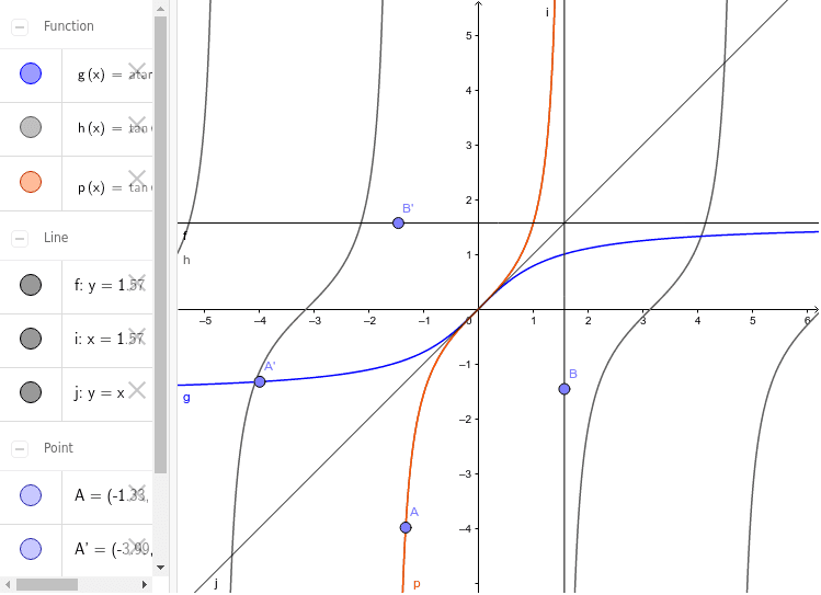
Dans un repère cartésien orthonormé du plan, la courbe représentative de la fonction arc tangente est obtenue à partir de la courbe représentative de la restriction de la fonction tangente à l'intervalle ${\displaystyle \left]-{\frac {\pi }{2}},{\frac {\pi }{2}}\right[}$ par une réflexion d'axe la droite d'équation y = x (puisqu'elle en est la fonction réciproque).

Parité

La fonction arctan est impaire, c'est-à-dire que (pour tout réel x) ${\displaystyle \arctan(-x)=-\arctan x}$.

Dérivée

Comme dérivée d'une fonction réciproque, arctan est dérivable et vérifie : ${\displaystyle \arctan '(x)={\frac {1}{1 x^{2}}}}$.

Développement en série de Taylor

Le développement en série de Taylor de la fonction arc tangente est :

${\displaystyle \forall x\in [-1,1]\quad \arctan x=\sum _{k=0}^{\infty }(-1)^{k}{\frac {x^{2k 1}}{2k 1}}=x-{\frac {1}{3}}x^{3} {\frac {1}{5}}x^{5}-{\frac {1}{7}}x^{7} \cdots }$.

Cette série entière converge vers arctan quand |x| ≤ 1 et x ≠ ±i. La fonction arc tangente est cependant définie sur tout ℝ (et même — cf. § « Fonction réciproque » — sur un domaine du plan complexe contenant à la fois ℝ et le disque unité fermé privé des deux points ±i).

Voir aussi Fonction hypergéométrique#Cas particuliers.

La fonction arctan peut être utilisée pour calculer des approximations de π ; la formule la plus simple, appelée formule de Leibniz, est le cas x = 1 du développement en série ci-dessus :

${\displaystyle {\frac {\pi }{4}}=1-{\frac {1}{3}} {\frac {1}{5}}-{\frac {1}{7}} \ldots }$.

Équation fonctionnelle

On peut déduire arctan(1/x) de arctan x et inversement, par les équations fonctionnelles suivantes :

${\displaystyle \forall x\in \mathbb {R} _{ }^{*}\quad \arctan {\frac {1}{x}} \arctan x={\frac {\pi }{2}}}$ ;

${\displaystyle \forall x\in \mathbb {R} _{-}^{*}\quad \arctan {\frac {1}{x}} \arctan x=-{\frac {\pi }{2}}}$.

Fonction réciproque

Par définition, la fonction arc tangente est la fonction réciproque de la restriction de la fonction tangente à l'intervalle ${\displaystyle \left]-{\frac {\pi }{2}},{\frac {\pi }{2}}\right[}$ : ${\displaystyle \forall x\in \mathbb {R} \quad y=\arctan x\iff \tan y=x{\text{ et }}y\in \left]-{\frac {\pi }{2}},{\frac {\pi }{2}}\right[}$.

Ainsi, pour tout réel x, tan(arctan x) = x. Mais l'équation arctan(tan y) = y n'est vérifiée que pour y compris entre ${\displaystyle -{\frac {\pi }{2}}}$ et ${\displaystyle {\frac {\pi }{2}}}$.

Dans le plan complexe, la fonction tangente est bijective de ]–π/2, π/2[ iℝ dans ℂ privé des deux demi-droites ]–∞, –1]i et [1, ∞[i de l'axe imaginaire pur, d'après son lien avec la fonction tangente hyperbolique et les propriétés de cette dernière. La définition ci-dessus de arctan s'étend donc en : ${\displaystyle \forall x\in \mathbb {C} \setminus {\big (}{\rm {i}}\left(]-\infty ,-1]\cup [1, \infty [\right){\big )}\quad y=\arctan x\iff \tan y=x{\text{ et }}y\in \left]-{\frac {\pi }{2}},{\frac {\pi }{2}}\right[ {\rm {i}}~\mathbb {R} }$.

Logarithme complexe

Par construction, la fonction arctangente est reliée à la fonction argument tangente hyperbolique et s'exprime donc, comme elle, par un logarithme complexe :

${\displaystyle \forall x\in \mathbb {C} \setminus \left({\rm {i}}\left(]-\infty ,-1]\cup [1, \infty [\right)\right)\quad \arctan x={\frac {1}{\rm {i}}}\operatorname {artanh} ({\rm {i}}x)={\frac {1}{2{\rm {i}}}}\ln {\frac {1 {\rm {i}}x}{1-{\rm {i}}x}}={\frac {\ln(1 {\rm {i}}x)-\ln(1-{\rm {i}}x)}{2{\rm {i}}}}}$.

Intégration

Primitive

La primitive de la fonction arc tangente qui s'annule en 0 s'obtient grâce à une intégration par parties :

${\displaystyle \int _{0}^{x}\arctan t\;\mathrm {d} t=x\,\arctan x-{\frac {1}{2}}\ln \left(1 x^{2}\right)}$.

Utilisation de la fonction arc tangente

La fonction arc tangente joue un rôle important dans l'intégration des expressions de la forme

${\displaystyle {\frac {1}{ax^{2} bx c}}}$

Si le discriminant D = b² – 4ac est positif ou nul, l'intégration est possible en revenant à une fraction partielle. Si le discriminant est strictement négatif, on peut faire la substitution par

${\displaystyle u={\frac {2ax b}{\sqrt {|D|}}}}$

qui donne pour l'expression à intégrer

${\displaystyle {\frac {4a}{|D|}}~{\frac {1}{1 u^{2}}}.}$

L'intégrale est alors

${\displaystyle {\frac {2}{\sqrt {|D|}}}\arctan {\frac {2ax b}{\sqrt {|D|}}}}$.

Formule remarquable

Si xy ≠ 1, alors :

${\displaystyle \arctan x \arctan y=\arctan {\frac {x y}{1-xy}} k\pi }$

où

${\displaystyle k={\begin{cases}0&{\text{si }}xy<1,\\1&{\text{si }}xy>1{\text{ avec }}x{\text{ (et }}y{\text{) }}>0,\\-1&{\text{si }}xy>1{\text{ avec }}x{\text{ (et }}y{\text{) }}<0.\end{cases}}}$

Autres utilisations

La forme en S de cette fonction fait qu'elle fait partie des fonctions dites sigmoïdes^{[citation nécessaire]}. Par rapport à la fonction logistique de Verhulst et la fonction erf, elle est celle qui est la plus lisse, c'est-à-dire celle qui est la plus longue à rejoindre ses asymptotes.

Notes et références

Voir aussi

Articles connexes

• Atan2
• Fonction circulaire réciproque
• L'arc tangente de tout rationnel non nul est irrationnel.
• Définition de la fonction arc tangente sur les complexes

Lien externe

(en) Eric W. Weisstein, « Inverse Tangent », sur MathWorld

• Portail de la géométrie
• Portail de l'analyse